Tutorial II: Custom Filters

The dpEmu package provides many filters for common use cases, but it might occur that no built-in filter exists for what you want. To solve this problem, you can create your own filters by inheriting the Filter-template. In this tutorial, we will create a custom filter for converting input images from RGB to grayscale.

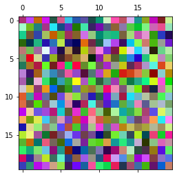
First, let’s generate some input data. We’ll use numpy’s randomstate with a set seed to ensure repeatability. The randomstate object simply replaces the np.random-part of any function call you want to make to numpy’s random module.

import matplotlib.pyplot as plt
import numpy as np

rand = np.random.RandomState(seed=0)
img = rand.randint(low=0, high=255, size=(20, 20, 3))
data = np.array([img for _ in range(9)])

Let’s see what these random images look like:

plt.matshow(data[0])

<matplotlib.image.AxesImage at 0x7fa3a2a4b0d0>

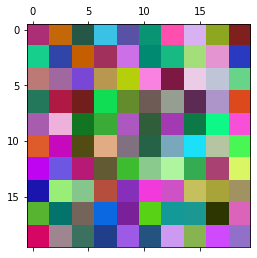
Before we write our own filter, let’s rehearse what we learned in the previous tutorial and try modifying the image with an existing filter. We’ll use the Resolution filter here.

from dpemu.nodes import Array, Series
from dpemu.filters.image import Resolution

image_node = Array()
series_node = Series(image_node)
resolution_filter = Resolution("scale")
image_node.addfilter(resolution_filter)

params = {"scale" : 2}
errorified = series_node.generate_error(data, params)

Let’s quickly check that the output is what we’d expect:

plt.matshow(errorified[0])

<matplotlib.image.AxesImage at 0x7fa3d6ff9590>

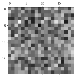
Now we’re ready to write our own filter to replace the built-in resolution filter. To do this, we want to inherit the Filter-class in dpemu.filters.filter. When we inherit the class, we’ll want to define a constructor and override the apply-function which applies the filter to the input data. The first parameter of the function is the input data. In this case we do not need the other two parameters, but we’ll learn how to use them later on in this tutorial.

from dpemu.filters.filter import Filter

class Grayscale(Filter):
    def __init__(self):
        super().__init__()
    def apply(self, node_data, random_state, named_dims):
        avg = np.sum(node_data, axis=-1) // 3
        for ci in range(3):
            node_data[:, :, ci] = avg

The code here is very simple. In the apply-function, we just take the mean of the color channels, and then assign that to each of them. Note that Filters must always maintain the dimensions of the input data. That is why the processed image will still contain 3 color channels, despite being in grayscale.

Let’s try our filter. Unlike before, we do not pass any parameters when calling generate_error, since or filter doesn’t take any parameters.

image_node = Array()
series_node = Series(image_node)
grayscale_filter = Grayscale()
image_node.addfilter(grayscale_filter)

params = {}
errorified = series_node.generate_error(data, params)

plt.matshow(errorified[0])

<matplotlib.image.AxesImage at 0x7fa397cff7d0>

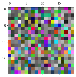
Now that we understand how a simple filter works, let’s incorporate randomness and parameters. We’ll change the filter so that every pixel gets replaced with its grayscale equivalent with some probability given as a parameter:

class RandomGrayscale(Filter):
    def __init__(self, probability_id):
        super().__init__()
        self.probability_id = probability_id
    def apply(self, node_data, random_state, named_dims):
        inds = random_state.rand(node_data.shape[0], node_data.shape[1]) < self.probability
        avg = np.sum(node_data[inds], axis=-1) // 3
        for ci in range(3):
            node_data[inds, ci] = avg

If you read the code carefully, you might notice that self.probability is not defined anywhere. For convenience, for every variable ending in _id, a value will be assigned to the variable without the _id-suffix from the params-list passed to generate_error. For example, if we have variable probability_id, which is set to "probability" in the initializer, and we call generate_error with a dictionary containing the key-value pair "probability" : 0.5, the value of self.probability will be 0.5.

In function __init__, we take the identifier for our probability parameter. This will be used as the key to find the value of self.probability from the params-dictionary.

In apply, we randomize the positions where the pixel will be replaced by its grayscale equivalent, then replace them as we did previously. For repeatability, we use the numpy RandomState passed to the function as the second parameter.

Let’s inspect the results:

image_node = Array()
series_node = Series(image_node)
grayscale_filter = RandomGrayscale("probability")
image_node.addfilter(grayscale_filter)

params = {"probability" : 0.5}
errorified = series_node.generate_error(data, params)

plt.matshow(errorified[0])

<matplotlib.image.AxesImage at 0x7f9c692bb160>

Now, the only thing we are yet to understand is the named_dims parameter to apply. For this, imagine our tuple of ten images is a video. We’ll create a filter that makes the pixels in the video decay into grayscale over time. Once a pixel turns grayscale, it won’t turn back, and by expectation half of the pixels will decay in the amount of frames given as a parameter.

Most of the new code is just randomizing the times at which individual pixels decay. Note that we make a copy of the random_state to ensure that we generate the same times for every image in the series. This is to ensure pixels don’t gain back their colors after decaying.

from math import log
from copy import deepcopy

class DecayGrayscale(Filter):
    def __init__(self, half_time_id):
        super().__init__()
        self.half_time_id = half_time_id
    def apply(self, node_data, random_state, named_dims):
        shape = (node_data.shape[0], node_data.shape[1])
        times = deepcopy(random_state).exponential(scale=(self.half_time / log(2)), size=shape)
        inds = times <= named_dims["time"]
        avg = np.sum(node_data[inds], axis=-1) // 3
        for ci in range(3):
            node_data[inds, ci] = avg

We use named_dims on the line inds = times <= named_dims["time"]. This line creates a mask of all pixels that decay before the current time, which is given by named_dims["time"]. To use this filter, we’ll have to tell the series-node that the dimension it is iterating over is called “time”:

image_node = Array()
series_node = Series(image_node, "time")
grayscale_filter = DecayGrayscale("half_time")
image_node.addfilter(grayscale_filter)

params = {"half_time" : 2}
errorified = series_node.generate_error(data, params)

Finally, to show multiple images in the same plot, we’ll have to do some more work:

fig = plt.figure(figsize=(8, 8))
for i in range(1, 9 + 1):
    fig.add_subplot(3, 3, i)
    plt.imshow(errorified[i-1])
plt.show()

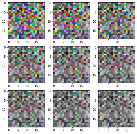
And we have achieved the desired effect! This concludes the second tutorial.

The notebook for this tutorial can be found here.