How dpEmu works
dpEmu consists of three components:
A system for building error generators
A system for running ML models with different error parameters
Tools for visualizing the results
Error Generation
For a quick hands-on introduction to error generation in dpEmu, see the Error Generation Basics tutorial.
Error generation in dpEmu consists of three simple steps:
Defining the structure of the data by constructing an error generation tree.
Attaching filters (error sources) to the tree.
Calling the
generate_errormethod on the root node of the tree.
Creating an Error Generation Tree
Error generation trees consist of tree nodes. The most common type of leaf node
is the Array, which can represent a Numpy array (or Python list) of any
dimension. Even a scalar value can be represented by an Array node provided
that node is not the root of the tree. If the fundamental unit of your data is
a tuple (as is the case with, e.g. .wav audio data), use a Tuple node as the
leaf.
The simplest and most commonly used non-leaf node type is the Series.
The Series represents the leftmost dimension of any unit of data passed to
it. For example, you might choose to represent a matrix of data as a series of
rows. In that case you would then create an Array node to represent a row
and provide it as the argument to a Series node:
from dpemu.nodes import Array, Series

row_node = Array()
root_node = Series(row_node)
A TupleSeries represents a tuple where the first (i.e. leftmost) dimensions of the tuple elements are in some sense “the same”. For example, if we have one Numpy array, X, containing the input data and another, Y, containing each data point’s correct label, we may choose to represent (X, Y) as a TupleSeries.
There is usually more than one valid way to represent the structure of the data as a tree. For example, a 2d Numpy array can be represented as:
a matrix, i.e. a single Array node
a list of rows, i.e. a Series with an Array as its child
a list of lists of scalars, i.e. a Series whose child is a Series whose child is an Array.
Adding Filters (Error Sources)
Filters can be added to leaf nodes such as Array or Tuple nodes.
Dozens of filters (e.g. Snow, Blur and SensorDrift) are provided
out of the box. They can be used to manipulate practically any kind of data,
including but not limited to images,time series and sound. Users can also
create their own custom error sources by subclassing the Filter class.
To create a filter, call the constructor and provide string identifiers for
the error parameters of that filter. To attach the filter to a leaf node,
call the node’s addfilter method with the filter object as the parameter.
Calling the generate_error Method
Once you have defined your error generation tree and added the desired filters,
you can call the generate_error method of the root node of the tree. The
method takes two arguments:
the data into which the errors are to be introduced, and
a dictionary of error parameters.
The parameter dictionary contains the error parameter values that are to be used in the error generation. The keys corresponding to the values are the error parameter identifier strings which you provided to the Filter constructor(s).
The generate_error method does not overwrite the original data but returns
a copy instead.
This is an example of what the error generation process might look like:
1 2 3 4 5 6 7 8 9 10 11 12 13 14 15 16 17 18 19 20 21 22 23 24 25 26 27 28 29 30 31 32 33 34 35 36 | import numpy as np
from dpemu.filters.common import Missing
from dpemu.nodes import Array, TupleSeries
# Assume our data is a tuple of the form (x, y) where x has
# shape (100, 10) and y has shape (100,). We can think of each
# row i as a data point where x_i represents the values of the
# explanatory variables and y_i represents the corresponding
# value of the response variable.
x = np.random.rand(100, 10)
y = np.random.rand(100, 1)
data = (x, y)
# Build a data model tree.
x_node = Array()
y_node = Array()
root_node = TupleSeries([x_node, y_node])
# Suppose we want to introduce NaN values (i.e. missing data)
# to y only (thus keeping x intact).
probability = .3
y_node.addfilter(Missing("p", "missing_val"))
# Feed the data to the root node.
output = root_node.generate_error(data, {'p': probability, 'missing_val': np.nan})
print("Output type (should be tuple):", type(output))
print("Output length (should be 2):", len(output))
print("Shape of first member of output tuple (should be (100, 10)):",
output[0].shape)
print("Shape of second first member of output tuple (should be (100,)):",
output[1].shape)
print("Number of NaNs in x (should be 0):",
np.isnan(output[0]).sum())
print(f"Number of NaNs in y (should be close to {probability * y.size}):",
np.isnan(output[1]).sum())
|
In the example the error generation tree has a TupleSeries as its
root node, which in turn has two Array nodes as its children. Then on
line 19 we add a Missing filter to one of the children, which will
transform some of the values in the 1-dimensional array y to NaN.
The filter is given a parameter with value “p”, which means that the key
for the probability for transforming a number into NaN is going to be
“p” in the parameter dictionary.
We then create a GaussianNoise filter and attach it to x_node, the
other child of the root node. The GaussianNoise filter takes two string
identifier arguments, corresponding to the mean and standard deviation
of the Gaussian distribution from which the noise is drawn.
Finally we call the generate_error method of the root node, providing
it with the data and the error parameter dictionary. The method returns
an errorified copy of the data. However, if you wish to run a machine
learning model on the data, the ML runner – to be discussed next – will
call the method for you.
ML runner system
The ML runner system, or simply runner, is a system which is used for running
multiple machine learning models simultaneously with distinct filter error
parameters by using multithreading. After running all the models with all
desired parameter combinations the system returns a pandas.DataFrame
object which can be used for visualizing the results.
The runner needs to be given the following values when it is run: train data, test data, a preprocessor, an error generation tree, a list of error parameters, a list of ML models and their parameters and a boolean indicating whether or not to use interactive mode.
Train data and test data
These are the original train data and test data which will be given to the ML
models. A None value can also be passed to the runner if there is no
training data.
Preprocessor
The preprocessor needs to implement a function run(train_data, test_data)
and it returns the preprocessed train and test data. The preprocessor can
return additional data as well, and it will be listed as separate columns in
the DataFrame which the runner returns.
Here is a simple example of a preprocessor, which does nothing to the original
data, but returns also an array called “negative_data” which contains the
additive inverse of each test_data’s element.
1 2 3 4 5 6 7 | class Preprocessor:
def __init__(self):
self.random_state = RandomState(42)
def run(self, train_data, test_data):
negative_data = -test_data
return train_data, test_data, {"negative_data": negative_data}
|
Error generation tree
The root node of the error generation tree should be given to the runner. The structure of the error generation tree is described above.
Error parameter list
The list of error parameters is simply a list of dictionaries which contain the keys and error values for the error generation tree.
AI model parameter list
The list of AI model parameters is a list of dictionaries containing three keys: “model”, “params_list” and “use_clean_train_data”.
The value of “model” is a class instead of an object.
The given class should implement the function run(train_data, test_data,
parameters) which runs the model on the train data and test data with given
parameters and returns a dictionary containing the scores and possibly
additional data.
The value of “params_list” is a list of dictionaries where each dictionary
contains one set of parameters for model. The model will be given these
parameters when the run(train_data, test_data, parameters) function is
called.
If the “use_clean_train_data” boolean is true, then no error will be added to the train data.
Here is an example AI model parameter list and a model:
1 2 3 4 5 6 7 8 9 10 11 12 13 14 15 16 17 18 19 20 21 22 23 24 25 26 27 28 29 30 | from numpy.random import RandomState
from sklearn.cluster import KMeans
from sklearn.metrics import adjusted_rand_score
from sklearn.metrics import adjusted_mutual_info_score
# Model
class KMeansModel:
def __init__(self):
self.random_state = RandomState(42)
def run(self, train_data, test_data, model_params):
labels = model_params["labels"]
n_classes = len(np.unique(labels))
fitted_model = KMeans(n_clusters=n_classes,
random_state=self.random_state
).fit(test_data)
return {
"AMI": round(adjusted_mutual_info_score(labels,
fitted_model.labels_,
average_method="arithmetic"),
3),
"ARI": round(adjusted_rand_score(labels, fitted_model.labels_), 3),
}
# Parameter list
model_params_dict_list = [
{"model": KMeansModel, "params_list": [{"labels": labels}]}
]
|
Interactive mode
The final parameter of the runner system is a boolean indicating whether to use interactive mode or not. Some of the functions for visualizing the results require interactive mode; for others it is optional. Most visualization functions have no interactive functionality.
Basically what the interactive mode does is that it adds a column containing
the modified test data to the resulting DataFrame object. The interactive
visualizer functions use this data to display points of data so that e.g.
the user can try to figure out why something was classified incorrectly.
Visualization functions
The dpemu.plotting_utils module contains several functions for plotting and
visualizing the data.
A Complete Example
Here is an unrealistic but simple example which demonstrates all three components of dpEmu. In this example we are trying to predict the next value of data when we know all earlier values in the data. Our model tries to do estimate this by keeping a weighted average. In the end of the example a plot of scores is visualized.
1 2 3 4 5 6 7 8 9 10 11 12 13 14 15 16 17 18 19 20 21 22 23 24 25 26 27 28 29 30 31 32 33 34 35 36 37 38 39 40 41 42 43 44 45 46 47 48 49 50 51 52 53 54 55 56 57 58 59 60 61 62 63 64 65 66 67 68 69 70 71 72 73 74 75 76 77 78 79 80 81 82 83 84 85 86 87 88 89 90 91 92 93 94 95 96 97 98 99 100 101 102 103 104 105 106 107 108 | import sys
import matplotlib.pyplot as plt
import numpy as np
from dpemu import runner
from dpemu.plotting_utils import visualize_scores, print_results_by_model, visualize_best_model_params
from dpemu.nodes import Array
from dpemu.filters.common import GaussianNoise
class Preprocessor:
def run(self, train_data, test_data, params):
return train_data, test_data, {}
class PredictorModel:
def run(self, train_data, test_data, params):
# The model tries to predict the values of test_data
# by using a weighted average of previous values
estimate = 0
squared_error = 0
for elem in test_data:
# Calculate error
squared_error += (elem - estimate) * (elem - estimate)
# Update estimate
estimate = (1 - params["weight"]) * estimate + params["weight"] * elem
mean_squared_error = squared_error / len(test_data)
return {"MSE": mean_squared_error}
def get_data(argv):
train_data = None
test_data = np.arange(int(sys.argv[1]))
return train_data, test_data
def get_err_root_node():
# Create error generation tree that has an Array node
# as its root node and a GaussianNoise filter
err_root_node = Array()
err_root_node.addfilter(GaussianNoise("mean", "std"))
return err_root_node
def get_err_params_list():
# The standard deviation goes from 0 to 20
return [{"mean": 0, "std": std} for std in range(0, 21)]
def get_model_params_dict_list():
# The model is run with different weighted estimates
return [{
"model": PredictorModel,
"params_list": [{'weight': w} for w in [0.0, 0.05, 0.15, 0.5, 1.0]],
"use_clean_train_data": False
}]
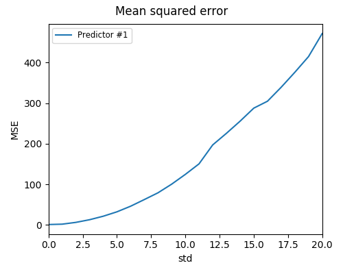
def visualize(df):
# Visualize mean squared error for all used standard deviations
visualize_scores(
df=df,
score_names=["MSE"],
is_higher_score_better=[False],
err_param_name="std",
title="Mean squared error"
)
visualize_best_model_params(
df=df,
model_name="Predictor #1",
model_params=["weight"],
score_names=["MSE"],
is_higher_score_better=[False],
err_param_name="std",
title=f"Best model params"
)
plt.show()
def main(argv):
# Create some fake data
if len(argv) == 2:
train_data, test_data = get_data(argv)
else:
exit(0)
# Run the whole thing and get DataFrame for visualization
df = runner.run(
train_data=train_data,
test_data=test_data,
preproc=Preprocessor,
preproc_params=None,
err_root_node=get_err_root_node(),
err_params_list=get_err_params_list(),
model_params_dict_list=get_model_params_dict_list()
)
print_results_by_model(df)
visualize(df)
if __name__ == "__main__":
main(sys.argv)
|
Run the program with the command:
python3 examples/run_manual_predictor_example 1000
Here’s what the resulting image should look like: